How format painter works in Excel

Have you ever encountered a situation where your boss threw you a task to correct the formatting on a spreadsheet just 15 minutes before an important meeting where the spreadsheet is to be presented? Or have you ever received an ugly spreadsheet from your co-workers when its aesthetic is unacceptable to you? Lucky you, in this article, I will introduce one magical tool in excel to you: the format painter. 

Where is the format painter located?

The format painter is an icon that looks like a paintbrush that can be found in the Home tab, clipboard section of the ribbon of Excel.

How to use the format painter?

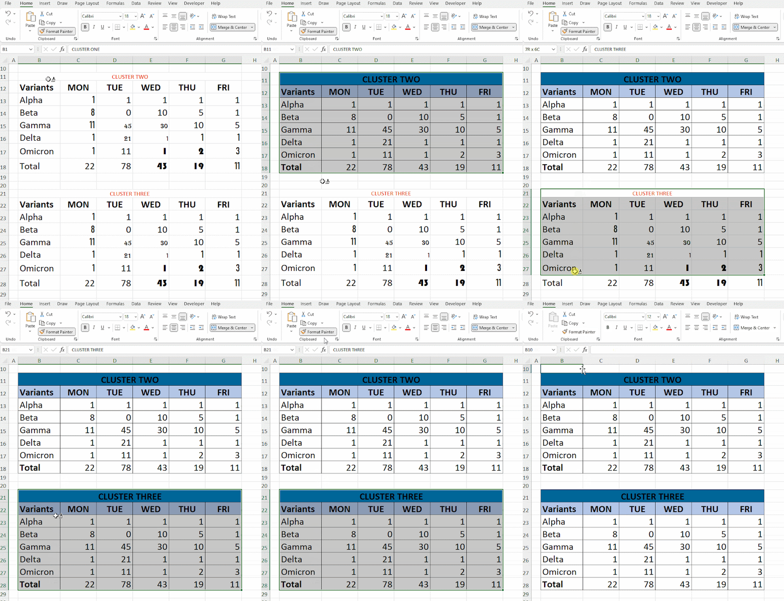
Let me use an example to show you how you can use the format painter. In the example below, there are two tables, namely Cluster One and Cluster Two. Both tables show the number of Covid patients grouped into different Covid variants by weekday. The Cluster One table is formatted aesthetically whereas the Cluster Two table is in its raw form. I shall walk you through step by step.

Step 1: Highlight the whole table Cluster One

Step 2: Click on the Format Painter icon

Step 3: Select the cell range in table Cluster Two you would like to apply the formatting, thereafter, release the mouse

And BOOM! Cluster Two table has been formatted.

If there is more than one area of the spreadsheet to apply the formatting to, the above method required you to click on the format painter each time to apply the formatting. 

For now, I will show you how you can use the format painter more efficiently if there is more than a single area of the spreadsheet to apply the formatting to. You can double-click on the format painter once to turn on the format painter mode, thereafter you can continue to apply the formatting to other areas and once you are done, you can turn off the format painter mode.

Here's how :

Step 1: Highlight the whole table Cluster One

Step 2: Double-Click the Format Painter icon to turn on the Format Painter mode. (Note: Mouse cursor should turn into a paintbrush icon.) 

Step 3: Select the cell range in table Cluster Two you would like to apply the formatting

Step 4: Continue selecting the cell range in table Cluster Three you would like to apply the formatting

Step 5: Click on the Format Painter icon to turn off the Format Painter mode

And now, you have the two raw tables formatted.

When to use format painter?

1. Applying consistent formatting for all different tables of a spreadsheet or of multiple spreadsheets.

2. Applying consistent formatting to rows and columns (eg. font typeface, font sizes, colours).

3. Applying consistent width or height of columns and rows.

4. Applying consistent formatting to shapes.

5. Applying consistent formatting to dates.

Why format painter does not work at times?

Format painter will not work on charts in Excel, this is one thing you have to note. You have to use the Paste Special function instead to apply consistent formatting for charts in Excel.

If you are trying to apply format consistency between cells that contain dates, be very careful that all the cell formats need to be in the date form. Format painter won't work if you try to use the format painter on the value that visibly looks like a date but in fact, it is a text format cell.

Hotkeys for format painter?

You can do the following :

Step1: Select the cell or range containing the desired format

Step 2: On your keyboard, press Alt, H, F, P 

Step 3: Click on the target cell or range you want to apply the formatting

One thing to take note of is that the shortcut keys have to be pressed one by one and not all at once.

Conclusion

By using this magical format painter tool, you will never ever find formatting a chore. It allows you to work with your spreadsheet more efficiently. 

Do check out the video at the top of this article if you would like to see in action what I have shared.